The Probability Theory of Prompts: Why Context Rewrites the Output Distribution

Stop talking to Large Language Models. They do not understand you, they do not care about your conversational tone, and they do not “think” about the problem.

An LLM is a conditional probability estimation engine. When you write a prompt, you are not giving instructions to an assistant. You are defining the boundary conditions of a high-dimensional probability space. Understanding this mathematical reality is the difference between hoping for a good response and deterministically Engineering one.

The LLM as a Probability Distributor

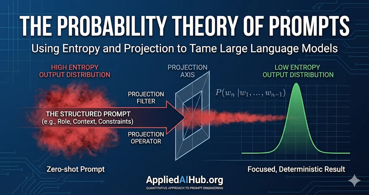
At its mathematical foundation, an autoregressive language model is constantly solving one problem: estimating the conditional probability distribution $P(w_{n} | w_{1}, w_{2}, ..., w_{n-1})$ for the next token, $w_n$.

When your prompt is extremely short or vague—such as “summarize this text”—you are placing the model in a state of maximum entropy. In information theory, this highly flat probability distribution means the Information Gain is near zero. Without constraints, the model samples from the most mediocre, statistically average paths in its training data. This is why zero-shot, low-effort prompts reliably produce bland, generic corporate-speak. They are mathematically destined to.

The Prompt as a Projection Operator

To understand why precision matters, we have to look at the mechanics of the Transformer architecture. The core self-attention mechanism calculates relevance scores using this function:

$Attention(Q, K, V) = softmax\left(\frac{QK^T}{\sqrt{d_k}}\right)V$

When you input a prompt, you are constructing the Query matrix ($Q$). The model’s parameterized knowledge is encoded in the Keys ($K$) and Values ($V$). The dot product $Q K^T$ computes vectors of similarity.

In linear algebra, a projection operator is a linear transformation $\mathbf{P}$ that maps a vector space onto a lower-dimensional subspace, effectively stripping away orthogonal (irrelevant) components. A prompt acts precisely as a non-linear projection operator over the model’s latent space.

When you write a generic prompt, $Q$ is diffuse. The dot product $QK^T$ yields a very flat attention distribution across a massive landscape of generic tokens. The $softmax$ function preserves this flatness, pulling in low-confidence values from everywhere.

This explains why Role Prompting is so effective—and why it is completely misunderstood. When you prepend a prompt with, “Act as a senior quantitative actuary,” you are not asking the AI to “play make-believe.” Mathematically, you are applying a rigid projection operator. You force the model to project its vast, diffuse, trillion-parameter space onto a highly specific, low-dimensional submanifold—the subspace of actuarial science.

Once projected onto this subspace:

1. The prior probability $P(\text{Term})$ shifts fundamentally: The attention scores ($QK^T$) for specialized jargon (e.g., stochastic mortality vectors) skyrocket.
2. Orthogonal noise is suppressed: The weights for conversational filler or unrelated domain knowledge (e.g., Python web development) are pushed toward zero.

The Measure Theory of Prompting

We can view reliable prompting frameworks (like RTGO: Role, Task, Goal, Constraints) strictly through the lens of Measure Theory and topology:

• Role (The Projection): Defines the subspace or manifold on which all subsequent probability calculations will occur.
• Task & Context (The Kernel): Provides the Kernel Function ($K(x, y)$) to filter out ambient noise. It defines the “shape” of the acceptable answer.
• Constraints (The Boundaries): Designate “forbidden zones” in the probability space. When you say “Output strictly in valid JSON with no markdown formatting”, you are forcing the probability mass of all conversational tokens (like “Here is your JSON:”) to $0$.

Author’s Comments: Frontline Reality

When building enterprise AI agents, we do not rely on the model “understanding” the task. We rely on the probability of it hallucinating being forced to zero because we have clamped every possible degree of freedom. If you give a model room to guess, it will guess wrong.

Why “Downstream Purpose” Kills Entropy

In a previous guide, I wrote about the One Prompt Rule—the necessity of defining exactly what the output will be used for. There is a rigid mathematical basis for this.

If you ask for an analysis but hide who will read it, the model must calculate a weighted average across all possible audiences, from a middle schooler to a Fortune 500 CEO. This explodes the conditional entropy.

By explicitly injecting the downstream purpose (let’s call it $C$ for context), you add a powerful conditional variable to the equation. You move from estimating $H(X|Y)$ to estimating $H(X|Y, C)$. This drastic reduction in entropy forces the model into a narrow, deterministic trajectory.

The Cost of Ambiguity: Experimental Validation

Let’s look at the actual cost of ambiguity on the token distribution.

Case A (High Entropy): “Analyze this data.” The model’s probability distribution splits wildly. Will it output a text summary? Python code? A JSON array? The Top-1 Token prediction probability might hover around a mere 10%.

Case B (Low Entropy): “Act as a quantitative analyst. Extract the volatility indices from this data and format them as a valid JSON array.” By adding role (quantitative analyst) and constraint (JSON array), the Top-1 Token prediction probability immediately spikes to 90%+. There is no longer any ambiguity.

To visualize how constraints reshape a Markov chain, look at this simple Python simulation:

import numpy as np

# A simplified transition matrix: [Generic, Technical, Code]
transitions = np.array([
    [0.6, 0.3, 0.1], # State 1: Generic Prompt
    [0.1, 0.8, 0.1], # State 2: Persona Applied
    [0.0, 0.1, 0.9]  # State 3: Constraint Applied (e.g. JSON format)
])

# Simulate 5 steps from a generic start state
current_state = np.array([1.0, 0.0, 0.0])

for step in range(5):
    current_state = current_state.dot(transitions)
    print(f"Step {step+1} Probability Dist: {current_state}")

The run result is as follows:

Step 1: [0.6      0.3      0.1    ]
Step 2: [0.39     0.43     0.18   ]
Step 3: [0.277    0.479    0.244  ]
Step 4: [0.2141   0.4907   0.2952 ]
Step 5: [0.17753  0.48631  0.33616]

Decrypting the Results

This code simplifies the LLM’s vast probability space into a Markov chain with three states:

1. State 1 (Generic): The model generates filler words, safe corporative-speak, and unstructured text.
2. State 2 (Technical): The model outputs domain-specific terminology.
3. State 3 (Constraint): The model strictly adheres to a formatting constraint, like outputting JSON brackets.

The transitions matrix dictates the mathematical gravity of the model. If the model is currently in a “Generic” state, it has a 60% chance of staying there. But if it enters a “Constraint” state, it has a 90% chance of remaining trapped in that highly structured format.

By setting the initial condition to current_state = np.array([1.0, 0.0, 0.0]), we simulate a zero-shot, generic prompt (e.g., “Write me something about data”).

Look at the terrifying reality mapped out in the 5 steps of the simulation: Even after 5 tokens of generation, the model still has nearly an 18% mathematical probability of outputting generic nonsense. In a multi-billion parameter space, an 18% chance of divergence per token guarantees a severe hallucination or useless output within a paragraph. The model is guessing.

Now, imagine shifting the starting state. If you apply a rigid prompt framework (Role + Constraint), you forcefully initialize the state to [0.0, 0.0, 1.0]. Because the constraint state acts as a probability firewall (with a 90% self-transition rate), the chance of the model wandering back into generic fluff is instantly reduced to near-zero.

Take Control of the Distribution

Writing good prompts is not an art. It is applied probability. Stop treating the AI like an intern and start treating it like a high-dimensional equation that you have to balance.

If you want to experience how applying structured, mathematical constraints optimizes your probability distribution, stop typing into an empty chat box. Use our Prompt Scaffold tool to forcefully align the model’s output layer before it even generates the first token.

---

Related reading:

• The One Prompt Rule — The mathematical necessity of defining exactly what the output will be used for downstream.
• AI Doesn’t Think: How it Compresses Human Experience — Why fluency is an artifact of dataset compression, not human-like reasoning.
• The RTGO Prompt Framework — A structural application of Measure Theory parameters (Role, Task, Goal, Constraints) into an actionable daily template.
• 10 Prompt Mistakes Everyone Makes (And How to Fix Them) — A practical guide on how to ruthlessly eliminate high-entropy ambiguity from your prompts.